Prior elicitation for directing replication efforts

Brent Roberts suggests the replication movement solicit federal funding for the organization of federally-funded replication daisy chains. James Coyne suggests that the replication movement has already made a grave misstep by attempting to replicate findings that were always hopelessly preposterous. Who is in the right?

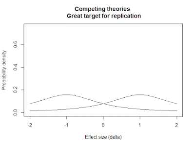
It seems to me that both are correct, but the challenge is in knowing when to replicate and when to dismiss outright. Coyne and the OSF seem to be after different things: the OSF has been very careful to make the RP:P about "estimating the replicability of psychology" in general rather than establishing the truth or falsity of particular effects of note. This motivated their decision to choose a random-ish sample of 100 studies rather than target specific controversial studies.

If in contrast, we want to direct our replication efforts to where they will have the greatest probative value, we will need to first identify which phenomena we are collectively most ambivalent about. There's no point in replicating something that's obviously trivially true or blatantly false.

How do we figure that out? Prior elicitation! We gather a diverse group of experts and ask them to divide up their probability, indicating how big they think the effect size is in a certain experimental paradigm.

If most the probability mass is away from zero, then we don't bother with the replication -- everybody believes in the effect already.

On the other hand, if the estimates are tightly clustered around zero, we don't bother with the replication -- it's obvious nobody believes it in the first place.

It's when the prior is diffuse, or evenly divided between the spike at zero and the slab outside zero, or bimodal, that we find the topic is controversial and in need of replication. That's the kind of thing that might benefit from a RRR or a federally-funded daisy chain.


Code below:
# Plot1
x = seq(-2, 2, .01)
plot(x, dcauchy(x, location = 1, scale = .3)*.9, type = 'l',
     ylim = c(0, 1),
     ylab = "Probability density",
     xlab = paste("Effect size (delta)"),
     main = "All-but-certain finding \n Little need for replication")
arrows(0, 0, 0, .1)

# Plot2
plot(x, dcauchy(x, location = 0, scale = .25)*.1, type = 'l',
     ylim = c(0, 1),
     ylab = "Probability density",
     xlab = paste("Effect size (delta)"),
     main = "No one believes it \n Little need for replication")
arrows(0, 0, 0, .9)

# Plot3
plot(x, dcauchy(x, location = 0, scale = 1)*.5, type = 'l',
     ylim = c(0, .75),
     ylab = "Probability density",
     xlab = paste("Effect size (delta)"),
     main = "No one knows what to think \n Great target for replication")
arrows(0, 0, 0, .5)

# Plot4
plot(x, dcauchy(x, location = 1, scale = 1)*.5, type = 'l',
     ylim = c(0, .75),
     ylab = "Probability density",
     xlab = paste("Effect size (delta)"),
     main = "Competing theories \n Great target for replication")
lines(x, dcauchy(x, location = -1, scale = 1)*.5)