Friday, November 28, 2014

Exciting New Misapplications of The New Statistics

This year's increased attention to effect sizes and confidence intervals (ESCI) has been great for psychological science. ESCI offers a number of improvements over null-hypothesis significance testing (NHST), such as an attention to practical significance and the elimination of dichotomous decision rules.

However, the problem of ESCI is that it is purely descriptive, not inferential. No hypotheses are named, and so ESCI doesn't report on the probability of a hypothesis given the data, or even the probability of the data given a null hypothesis. No process or statistic turns the ESCI into a decision, although we might make Geoff Cumming cringe by looking at whether the ESCI includes zero and making a decision based on that, thereby falling right back to using NHST.

The point is, there's no theoretical or even pragmatic method for turning an ESCI into an inference. At what point does a confidence interval become sufficiently narrow to make a decision? We know that values near the extremes of the interval are often less likely than the values near the middle, but how much less likely?

I'm not asking for a formal dichotomous decision rule (I'm a Bayesian, I have resigned my life to uncertainty), but I've already noticed the ways we can apply ESCI inconsistently to overstate the evidence. See a recent example from Boothby, Clark, and Bargh (PDF link), arguing that shared experiences are more intense in two studies of n = 23 women:
Indeed, our analyses indicated that participants liked the chocolate significantly less when the confederate was also eating the chocolate (M = 2.45, SD = 1.77) than when the confederate was reviewing the computational products (M = 3.16, SD = 2.32), t(21) = 2.42, p = .025, 95% CI for the difference between conditions = [0.10, 1.31], Cohen’s d = 0.34. Participants reported feeling more absorbed in the experience of eating the chocolate in the shared-experience condition (M = 6.11, SD = 2.27) than in the unshared-experience condition (M = 5.39, SD = 2.43), p = .14. Participants also felt like they were more “on the same wavelength” with the confederate during the shared-experience condition (M = 6.43, SD = 1.38) compared with the unshared-experience condition (M = 5.61, SD = 1.38), t(21) = 2.35, p = .03, 95% CI for the difference
between conditions = [0.10, 1.54], Cohen’s d = 0.59 (see Fig. 2). There were no significant differences in participants’ self-reported mood or any other feedback measures between the shared and the unshared-experience conditions (all ps > .10).
Normally one wouldn't be allowed to talk about that p = .14 as evidence for an effect, but we now live in a more enlightened ESCI period in which we're trying to get away from dichotomous decision making. Okay, that's great, although I'd question the wisdom of trying to make any inference based on such a small sample, even within-subjects. But notice that when p = .14 is in the direction of their expected effect, it is interpreted as evidence for the phenomenon, but when differences are in a direction that does not support the hypothesis, it is simply reported as "not significant, p > .10". If we're going to abandon NHST for ESCI, we should at least be consistent about reporting ALL the ESCIs, and not just the ones that support our hypotheses.

Or, better yet, use that ESCI to actually make a principled and consistent inference through Bayes Factor. Specify an alternative hypothesis of what the theory might suggest are likely effect sizes. In this example, one might say that the effect size is somewhere between d = 0 and d = 0.5, with smaller values more likely than large values. This would look like the upper half of a normal distribution with mean 0 and standard deviation .5. Then we'd see how probable the obtained effect is given this alternative hypothesis and compare it to how probable the effect would be given the null hypothesis. At 20 subjects, I'm going to guess that the evidence is a little less than 3:1 odds for the alternative for the significant items, and less than that for the other items.

ESCI's a good first step, but we need to be careful and consistent about how we use it before we send ourselves to a fresh new hell. But when Bayesian analysis is this easy for simple study designs, why stop at ESCI?

Tuesday, July 1, 2014

Can p-curve detect p-hacking through moderator trawling?

NOTE: Dr. Simonsohn has contacted me and indicated a possible error in my algorithm. The results presented here could be invalid. We are talking back in forth and I am trying to fix my code. Stay tuned!

Suppose a researcher were to conduct an experiment looking to see if Manipulation X had any effect on Outcome Y, but the result was not significant. Since nonsignificant results are harder to publish, the researcher might be motivated to find some sort of significant effect somehow. How might the researcher go about dredging up a significant p-value?

One possibility is "moderator trawling". The researcher could try potential moderating variables until one is found that provides a significant interaction. Maybe it only works for men but not women? Maybe the effect can be seen after error trials, but not after successful trials? In essence, this is slicing the data until one manages to find a subset of the data that does show the desired effect. Given the number of psychological findings that seem to depend on surprisingly nuanced moderating conditions (ESP is one of these, but there are others), I do not think this is an uncommon practice.

To demonstrate moderator trawling, here's a set of data that has no main effect.
However, when we slice up the data by one of our moderators, we do find an effect. Here the interaction is significant, and the simple slope in group 0 is also significant.

In the long run, testing the main effect and three moderators will cause the alpha error rate to increase from 5% to 18.5%. That's the chance that at least one of the four tests come up p>.05, (.95)^4.

Because I am intensely excited by the prospect of p-curve meta-analysis, I just had to program a simulation to see whether p-curve could detect this moderator trawling in the absence of a real effect. P-curve meta-analysis is a statistical technique which examines the distribution of reported significant p-values. It relies on the property of the p-value that, when the null is true, p is uniformly distributed between 0 and 1. When an effect exists, smaller p-values are more likely than larger p-values, even for small p: p < .01 is more likely than .04<p<.05 for a true effect. Thus, a flat p-curve indicates no effect and possible file-drawering of null findings, while a right-skewed p-curve indicates a true effect. More interesting yet, a left-skewed curve suggests p-hacking -- doing what you need to to achieve p < .05, alpha error be damned.

You can find the simulation hosted on Open Science Framework at https://osf.io/ydwef/. This is my first swipe at an algorithm; I'd be happy to hear other suggestions for algorithms and parameters that simulate moderator trawling. Here's what the script does.
1) Create independent x and y variables from a normal distribution
2) Create three moderator variables z1, z2, and z3, of which 10 random subjects make up each of two levels
3) Fit the main effect model y ~ x. If it's statistically significant, stop and report the main effect.
4) If that doesn't come out significant, try z1, z2, and z3 each as moderators (e.g. y ~ x*z1; y ~ x*z2; y ~ x*z3). If one of these is significant, stop and plan to report the interaction.
5) Simonsohn et al. recommend using the p-value of the interaction for an attenuation interaction (e.g. "There's an effect among men that is reduced or eliminated among women"), but the p-values of each of the simple slopes for a crossover interaction (e.g. "This makes men more angry but makes women less angry."). So, determine whether it's an attenuation or crossover interaction.
5a)  If just one simple slope is significant, we'll call it an interaction. There's an effect in one group that is significant that is eliminated or reduced in the other group. In this case, we report the interaction p-value.
5b) If neither simple slopes are significant, or both are significant with coefficients of opposite sign, we'll call it a crossover. Both slopes significant indicates opposite effects, while neither slope significant indicates that the simple slopes aren't strong enough on their own but their opposition is enough to power a significant interaction. In these cases, we'll report both simple slopes' p-values.

We repeat this for 10,000 hypothetical studies, export the t-tests, and put them into the p-curve app at www.p-curve.com. Can p-curve tell that these results are the product of p-hacking?


It cannot. In the limit, it seems that p-curve will conclude that the findings are very mildly informative, indicating that the p-curve is flatter than 33% power, but still right-skewed, suggesting a true effect measured at about 20% power. Worse yet, it cannot detect that these p-values come from post-hoc tomfoolery and p-hacking. A few of these sprinkled into a research literature could make an effect seem to bear slightly more evidence, and be less p-hacked, then it really is.

The problem would seem to be that the p-values are aggregated across heterogeneous statistical tests: some tests of the main effect, some tests of this interaction or that interaction. Heterogeneity seems like it would be a serious problem for p-curve analysis in other ways. What happens when the p-values come from a combination of well-powered studies of a true effect and some poorly-powered, p-hacked studies of that same effect? (As best I can tell from the manuscript draft, the resulting p-curve is flat!) How does one meta-analyze across studies of different phenomena or different operationalizations or different models?

I remain excited and optimistic for the future of p-curve meta-analysis as a way to consider the strength of research findings. However, I am concerned by the ambiguities of practice and interpretation in the above case. It would be a shame if these p-hacked interactions would be interpreted as evidence of a true effect. For now, I think it best to report the data with and without moderators, preregister analysis plans, and ask researchers to report all study variables. In this way, one can reduce the alpha-inflation and understand how badly the results seem to rely upon moderator trawling.

Tuesday, May 20, 2014

Psychology's Awkward Puberty

There's a theory of typical neural development I remember from my times as a neuroscience student. It goes like this: in the beginning of development, the brain's tissues rapidly grow in size and thickness. General-purpose cells are replaced with more specialized cells. Neurons proliferate, and rich interconnections bind them together.

Around the time of puberty, neurons start dying off and many of those connections are pruned. This isn't a bad thing, and in fact, seems to be good for typical neural development, since there seems to be an association between mental disorder and brains that failed to prune.

In the past half a century, psychological science has managed to publish an astonishing number of connections between concepts. For example, people experience physical warmth as interpersonal warmth, hot temperatures make them see more hostile behavior, eating granola with the ingredients all mixed up makes them more creative than eating granola ingredients separately, and seeing the national flag makes them more conservative. Can all of these fantastic connections be true, important, meaningful? Probably not.

Until now, psychology has been designed for the proliferation of effects. Our most common statistical procedure, null hypothesis significance testing, can only find effects, not prove their absence. Researchers are rewarded for finding effects, not performing good science, and the weirder the effect, the more excited the response. And so, we played the game, finding lots of real effects and lots of other somethings we could believe in, too.

It's now time for us to prune some connections. Psychology doesn't know too little, it knows too much -- so much that we can't tell truth from wistful thinking anymore. Even the most bizarre and sorcerous manipulations still manage to eke out p < .05 often enough to turn up in journals. "Everything correlates at r = .30!" we joke. "Everything! Isn't that funny?" One can't hear the truth, overpowered as it is by the neverending chorus of significance, significance, significance.

This pruning process makes researchers nervous, concerned that their effect which garnered them tenure, grants, and fame will be torn to shreds, leaving them naked and foolish. We must remember that the authors of unreplicable findings didn't necessarily do anything wrong -- even the most scrupulous researcher will get p < .05 one time in 20 in the absence of a true effect. That's how Type I error works. (Although one might still wonder how an effect could enjoy so many conceptual replications within a single lab yet fall to pieces the moment they leave the lab.)

Today, psychology finally enters puberty. It's bound to be awkward and painful, full of hurt feelings, awkwardness, and embarrassment, but it's a sign we're also gaining a little maturity. Let's look forward to the days ahead, in which we know more through knowing less.

Monday, March 24, 2014

Intuitions about p

Two of my labmates were given a practice assignment for a statistics class. Their assignment was to generate simulated data where there was no relationship between x and y. In R, this is easy, and can be done by the code below: x is just the numbers from 1:20, and y is twenty random pulls from a normal distribution.

dat=data.frame("x"=1:20,
               "y"=rnorm(20)
               )
m1 = lm(y ~ x, data=dat)
summary(m1)

One of my labmates ran the above code, frowned, and asked me where he had gone wrong. His p-value was 0.06 -- "marginally significant"! Was x somehow predicting y? I looked at his code and confirmed that it had been written properly and that there was no relationship between x and y. He frowned again. "Maybe I didn't simulate enough subjects," he said. I assured him this was not the case.

It's a common, flawed intuition among researchers that p-values naturally gravitate towards 1 with increasing power or smaller (more nonexistent?) effects. This is an understandable fallacy. As sample size increases, power increases, reducing the Type II error rate. It might be mistakenly assumed, then, that Type I error rate also reduces with sample size. However, increasing sample size does nothing to p-value when the null is true. When there is no effect, p-values come from a uniform distribution: a p-value less than .05 is just as likely as a p-value greater than .95!

As we increase our statistical power, the likelihood of Type II error (failing to notice a present effect) approaches zero. However, Type I error remains constant at whatever we set it to, no matter how many observations we collect. (You could, of course, trade power for a reduction in Type I error by setting a more stringent cutoff for "significant" p-values like .01, but this is pretty rare in our field where p<.05 is good enough to publish.)

Because we don't realize that p is uniformly distributed when the null is true, we overinterpret all our p-values that are less than about .15. We've all had the experience of looking at our data and being taunted by a p-value of 0.11. "It's so low! It's tantalizingly close to marginal significance already. There must be something there, or else it would have a really meaningless p-value like p=.26. I just need to run a few more subjects, or throw out the outlier that's ruining it," we say to ourselves. "This isn't p-hacking -- my effect is really there, and I just need to reveal it."

We say hopelessly optimistic things like "p = .08 is approaching significance." The p-value is doing no such thing -- it is .08 for this data and analysis, and it is not moving anywhere. Of course, if you are in the habit of peeking at the data and adding subjects until you reach p < .05, it certainly could be "approaching" significance, but that says more about the flaws of your approach to research than the validity of your observed effects.

How about effect size? Effect size, unlike p, benefits from increasing sample size whether there's an effect or not. As sample size is added, estimates of true effects approach their real value, and estimates of null effects approach zero. Of course, after a certain point the benefits of even more samples starts to decrease: going from n=200 to n=400 yields a bigger benefit to precision than does going from n=1000 to n=1200.

Let's see what effect size estimates of type I errors look like at small and large N.


Here's a Type I error at n=20. Notice that the slope is pretty steep. Here we estimate the effect size to be a whopping |r| = .44! Armed with only a p-value and this point estimate, a naive reader might be inclined to believe that the effect is indeed huge, while a slightly skeptical reader might round down to about |r| = .20. They'd both be wrong, however, since the true effect size is zero. Random numbers are often more variable than we think!


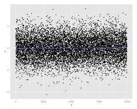
Let's try that again. Here's a Type I error at n = 10,000. Even though the p-value is statistically significant (here, p = .02), the effect size is pathetically small: |r| = .02. This is one of the many benefits of reporting the effect size and confidence interval. Significance testing will always be wrong at least 5% of the time, while effect size estimates will always benefit from power.

This is how we got the silly story about the decline effect (http://www.newyorker.com/reporting/2010/12/13/101213fa_fact_lehrer), in which scientific discoveries tend to "wear off" over time. Suppose you find a Type I error in your n=20 study. Now you go to replicate it, and since you have faith in your effect, you don't mind running additional subjects and re-analyzing until you find p < .05. This is p-hacking, but let's presume you don't care. Chances are it will take you more than 20 subjects before you "find" your Type I error again, because it's unlikely that you would be so lucky as to find the same Type I error within the first 20 subjects. By the point that you do find p < .05, you will probably have run rather more than 20 subjects, and so the effect size estimate will be a little more precise and be precipitously closer to zero. The truth doesn't "wear off." The truth always outs.

Of course, effect size estimates aren't immune to p-hacking, either. One of the serious consequences of p-hacking is that it biases effect sizes.

Collect big enough samples. Look at your effect sizes and confidence intervals. Report everything you've got in the way that makes the most sense. Don't trust p. Don't chase p.