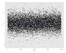
Two of my labmates were given a practice assignment for a statistics class. Their assignment was to generate simulated data where there was no relationship between x and y. In R, this is easy, and can be done by the code below: x is just the numbers from 1:20, and y is twenty random pulls from a normal distribution.
dat=data.frame("x"=1:20,
"y"=rnorm(20)
)
m1 = lm(y ~ x, data=dat)
summary(m1)
One of my labmates ran the above code, frowned, and asked me where he had gone wrong. His p-value was 0.06 -- "marginally significant"! Was x somehow predicting y? I looked at his code and confirmed that it had been written properly and that there was no relationship between x and y. He frowned again. "Maybe I didn't simulate enough subjects," he said. I assured him this was not the case.
It's a common, flawed intuition among researchers that p-values naturally gravitate towards 1 with increasing power or smaller (more nonexistent?) effects. This is an understandable fallacy. As sample size increases, power increases, reducing the Type II error rate. It might be mistakenly assumed, then, that Type I error rate also reduces with sample size. However, increasing sample size does nothing to p-value when the null is true. When there is no effect, p-values come from a uniform distribution: a p-value less than .05 is just as likely as a p-value greater than .95!
As we increase our statistical power, the likelihood of Type II error (failing to notice a present effect) approaches zero. However, Type I error remains constant at whatever we set it to, no matter how many observations we collect. (You could, of course, trade power for a reduction in Type I error by setting a more stringent cutoff for "significant" p-values like .01, but this is pretty rare in our field where p<.05 is good enough to publish.)
Because we don't realize that p is uniformly distributed when the null is true, we overinterpret all our p-values that are less than about .15. We've all had the experience of looking at our data and being taunted by a p-value of 0.11. "It's so low! It's tantalizingly close to marginal significance already. There must be something there, or else it would have a really meaningless p-value like p=.26. I just need to run a few more subjects, or throw out the outlier that's ruining it," we say to ourselves. "This isn't p-hacking -- my effect is really there, and I just need to reveal it."
We say hopelessly optimistic things like "p = .08 is approaching significance." The p-value is doing no such thing -- it is .08 for this data and analysis, and it is not moving anywhere. Of course, if you are in the habit of peeking at the data and adding subjects until you reach p < .05, it certainly could be "approaching" significance, but that says more about the flaws of your approach to research than the validity of your observed effects.
How about effect size? Effect size, unlike p, benefits from increasing sample size whether there's an effect or not. As sample size is added, estimates of true effects approach their real value, and estimates of null effects approach zero. Of course, after a certain point the benefits of even more samples starts to decrease: going from n=200 to n=400 yields a bigger benefit to precision than does going from n=1000 to n=1200.
Let's see what effect size estimates of type I errors look like at small and large N.
Here's a Type I error at n=20. Notice that the slope is pretty steep. Here we estimate the effect size to be a whopping |r| = .44! Armed with only a p-value and this point estimate, a naive reader might be inclined to believe that the effect is indeed huge, while a slightly skeptical reader might round down to about |r| = .20. They'd both be wrong, however, since the true effect size is zero. Random numbers are often more variable than we think!
Let's try that again. Here's a Type I error at n = 10,000. Even though the p-value is statistically significant (here, p = .02), the effect size is pathetically small: |r| = .02. This is one of the many benefits of reporting the effect size and confidence interval. Significance testing will always be wrong at least 5% of the time, while effect size estimates will always benefit from power.
This is how we got the silly story about the decline effect (http://www.newyorker.com/reporting/2010/12/13/101213fa_fact_lehrer), in which scientific discoveries tend to "wear off" over time. Suppose you find a Type I error in your n=20 study. Now you go to replicate it, and since you have faith in your effect, you don't mind running additional subjects and re-analyzing until you find p < .05. This is p-hacking, but let's presume you don't care. Chances are it will take you more than 20 subjects before you "find" your Type I error again, because it's unlikely that you would be so lucky as to find the same Type I error within the first 20 subjects. By the point that you do find p < .05, you will probably have run rather more than 20 subjects, and so the effect size estimate will be a little more precise and be precipitously closer to zero. The truth doesn't "wear off." The truth always outs.
Of course, effect size estimates aren't immune to p-hacking, either. One of the serious consequences of p-hacking is that it biases effect sizes.
Collect big enough samples. Look at your effect sizes and confidence intervals. Report everything you've got in the way that makes the most sense. Don't trust p. Don't chase p.


